Success Has Many Fathers: Attribution Without Identification#
Why credit models rank channels by diagnosticity, not by cause#
1. The problem#
Success has many fathers. Failure dies an orphan.
The proverb is normally read as a comment on human vanity. In marketing analytics it is a description of a data-generating process, and it is doing more damage than the vanity it describes.
A multi-touch attribution report shows that converting deals touched, on average, eleven channels. Credit is distributed across those eleven. Every channel appears to work. The budget conversation that follows is about reallocating fractions, and the fractions are defended with a model.
Then someone looks at the top-credited channel and finds it is the Contact Us form. The prospect arrived, typed their name, and asked to speak to sales. Attribution credits this heavily, because records that submit contact forms convert at extraordinary rates.
This is where the reasoning should stop and rarely does. The contact form did not cause the purchase. It revealed a purchase intention that already existed — an intention that also caused the prospect to open the emails, attend the webinar, and click the ad, all of which are now collecting credit for the same reason. The form is a thermometer, and attribution has credited it for the fever.
This note establishes that the failure is structural rather than a matter of choosing a better credit rule, identifies what attribution models actually measure, and states what would have to be true to measure the thing everyone believes they are measuring.
Relationship to TN-2026-002. The companion note concerns projection: one two-dimensional object, three lower-dimensional reports, information lost by marginalizing. This note concerns the assignment mechanism: the object is fine and the sampling is corrupted. The failure modes are orthogonal and they compound. Moving from period reports to cohort reports repairs the projection error and leaves the confounding entirely untouched — which matters, because “we switched to cohort analysis” is the standard false remedy.
2. The object#
Let $i$ index prospects. Each carries:
- a latent propensity $Z_i$ — budget, mandate, timing, incumbent pain. Unobserved, though partially proxied by firmographics and behavioural scores.
- a touch profile $T_i = (T_{i1}, \dots, T_{iK}) \in \mathbb{N}^K$, counts of exposure across $K$ channels.
- an outcome $Y_i \in \{0, 1\}$, conversion.
Following the potential-outcomes convention, let $Y_i(t)$ denote the outcome prospect $i$ would realise under touch profile $t$. The causal estimand for channel $k$ is the incremental effect
$$ \tau_k \;=\; \mathbb{E}\bigl[\, Y_i(T_i + e_k) - Y_i(T_i) \,\bigr], $$the change in conversion probability from one additional touch on channel $k$, holding everything else fixed. This is the quantity every budget decision requires and no attribution model returns.
2.1 The assignment mechanism#
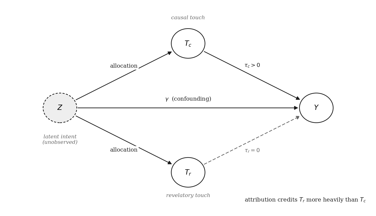
Touches are not randomly assigned. They are allocated by a scoring system:
$$ T_i \;\sim\; \pi\bigl(\cdot \mid \hat{Z}_i, H_{i}\bigr), $$where $\hat{Z}_i$ is the firm’s estimate of propensity and $H_i$ the observed history. Higher-scoring prospects receive more sequences, faster follow-up, better-qualified reps, and event invitations. This is not a defect in the marketing operation. It is the marketing operation working correctly.
But it means $Z$ causes both $T$ and $Y$. In the epidemiological literature this structure is called confounding by indication: treatment is allocated on the basis of the prognosis being measured. It is the mechanism that made a decade of observational hormone-replacement studies wrong — physicians prescribed to healthier patients, and the drug collected the credit.
2.2 Revelatory versus causal touches#
Definition. A channel $k$ is revelatory if $Z \to T_k$ and $\tau_k = 0$: exposure is caused by intent and has no effect on the outcome.
Contact-form submissions, pricing-page visits, branded search, documentation reads, and return visits to a comparison page are all substantially revelatory. They are measurements of $Z$ that have been recorded in the same table as treatments and are subsequently indistinguishable from them.
2.3 What attribution computes#
An attribution model is a credit rule mapping a converting path to a point on the simplex:
$$ c : \text{path} \longrightarrow \Delta^{K-1}, \qquad \sum_{k=1}^{K} c_k = 1. $$First-touch, last-touch, linear, time-decay, position-based, Markov-removal, and Shapley-value allocations are all of this form. They differ in how they spread the unit of credit and agree in spreading exactly one unit.
3. Results#
Proposition 1 (the simplex has no null)#
For any credit rule $c$ into $\Delta^{K-1}$, and any population in which $\tau_k = 0$ for every $k$, the model returns strictly positive aggregate credit to every channel appearing on converting paths.
Proof. Immediate from $\sum_k c_k = 1$. Every conversion distributes one unit of credit regardless of the underlying $\tau$. A channel receives zero only if another receives more. $\square$
The consequence is not a bias to be corrected. It is a statement about the model’s range. An estimator that cannot return “none of this worked” cannot distinguish a world where marketing works from one where it does not, and therefore carries no information about which world we are in. This disqualifies the entire family as causal estimators before any data is collected.
Shapley-value attribution deserves a specific note, because it is the version usually offered as the rigorous one. The Shapley value is the unique fair division of a fixed surplus among contributors. Its axioms — efficiency, symmetry, additivity — are axioms about allocation, and efficiency is exactly the constraint that the parts sum to the whole. It is a superb answer to “how should we divide the credit,” and answering that question well presupposes that credit is owed.
Proposition 2 (the bias is signed, and scoring amplifies it)#
Take the linear working model
$$ Y_i = \alpha + \beta T_i + \gamma Z_i + \varepsilon_i, \qquad T_i = \delta + \lambda Z_i + u_i, $$with $\gamma > 0$ (intent raises conversion) and $\lambda > 0$ (allocation is monotone in estimated intent). Then
$$ \operatorname*{plim} \hat{\beta}_{\text{OLS}} \;=\; \beta + \gamma\,\frac{\operatorname{Cov}(T, Z)}{\operatorname{Var}(T)} \;=\; \beta + \frac{\gamma \lambda \operatorname{Var}(Z)}{\lambda^{2}\operatorname{Var}(Z) + \operatorname{Var}(u)} \;>\; \beta . $$Three consequences, in increasing order of unwelcomeness.
The bias is upward, always. Whenever allocation responds positively to intent, observed channel effects exceed true effects. Attribution does not add symmetric noise around the truth; it overstates in a known direction. Any decision rule of the form “cut the lowest-credited channel” is therefore not merely noisy but systematically wrong about which channel is lowest.
The bias is largest where allocation is most responsive. Channels reserved for high-score prospects — SDR sequences, executive dinners, field events, account-based programmes — carry the largest inflation, precisely because they are the best targeted.
Improving the scoring model provably increases the bias. As targeting sharpens, $\lambda$ rises and $\operatorname{Var}(u)$ falls, so the bias term increases monotonically toward $\gamma$. In the limit of perfect targeting, $\operatorname{Var}(u) \to 0$ and the observed coefficient converges to $\beta + \gamma/\lambda$ regardless of $\beta$.
This is the result worth internalising. The two initiatives most revenue teams run in parallel — invest in lead scoring and invest in attribution — are in direct conflict. Each increment of targeting quality degrades the measurement system used to evaluate it. A firm that scores well and attributes carefully will produce more confident and more wrong numbers than one that does neither.
Proposition 3 (attribution ranks by diagnosticity)#
Under any recency- or proximity-weighted credit rule, the expected credit assigned to channel $k$ is increasing in the strength of association between $T_k$ and $Z$, holding $\tau_k$ fixed.
Sketch. Credit rules weight touches by proximity to conversion. A channel whose exposure is strongly driven by intent occurs disproportionately among high-$Z$ records, and among those records occurs disproportionately late, since intent is revealed progressively. Both effects raise expected credit independently of $\tau_k$. $\square$
So attribution orders channels by how informative they are about intent. That ordering is real and stable, and it is not the causal ordering. Under Proposition 3, a purely revelatory channel with $\tau_k = 0$ can and routinely does outrank a genuinely causal channel.
This reframes what the tooling is for. Attribution is a decent estimator of diagnosticity — a channel’s mutual information with $Z$ — which is a legitimate and valuable quantity. High-diagnosticity signals are exactly what should drive routing, prioritisation, and SDR queueing. The error is not in computing them. The error is in spending against them.
Proposition 4 (conditioning on success)#
Credit is allocated only along converting paths. Non-converting paths are recorded and discarded. The quantity a report aggregates is therefore
$$ P(T_k \mid Y = 1), $$the prevalence of a channel among successes. What the reader takes from the report is
$$ P(Y = 1 \mid T_k), $$the conversion rate given the channel. Bayes’ rule relates them:
$$ P(Y=1 \mid T_k) \;=\; \frac{P(T_k \mid Y=1)\, P(Y=1)}{P(T_k)} . $$The two coincide only when $P(T_k) = P(Y=1)$, which nothing enforces. A channel that touches nearly everything will appear on nearly every converting path and receive credit accordingly, while its conversion rate may be the base rate exactly.
This is the prosecutor’s fallacy wearing a dashboard, and it is the formal content of “success has many fathers.” Successes accumulate apparent parents because we count parents only at successes. The orphaned failures are the control group, and they have been deleted from the numerator and the denominator both.
4. What this does not cover#
Attribution retains legitimate uses. Coverage analysis (which segments no channel reaches), path diagnostics (where records stall), and routing priority all consume the diagnosticity ranking correctly. The objection in this note is narrow: attribution output must not be used to set budget.
The linear model in Proposition 2 is a working model. Real response is non-linear with saturation and interaction. The sign of the bias survives under any monotone allocation rule and monotone response, which is the claim being made; the closed-form magnitude does not.
Touches are not cleanly bipartite. The revelatory/causal distinction is a spectrum, not a partition. A product demo both reveals intent and persuades. The definition in §2.2 is a limiting case used to make the mechanism visible, and mixed channels require the decomposition to be estimated rather than assumed.
Competitive and equilibrium response is ignored. A channel with $\tau_k = 0$ in isolation may still be defensive — branded search is the canonical case, where the measured effect is near zero until a competitor bids on your name. Incrementality experiments run in a stable competitive environment do not price that option.
Selection into the CRM is not addressed. Everything here conditions on the prospect existing as a record. Whatever process determines that is upstream of this analysis and is very likely also intent-responsive.
5. Identification#
$\tau_k$ is identified when there exists variation in $T_k$ independent of $Z$ given observables. Four sources, in descending order of quality:
- Randomised holdout. A fraction of eligible records is withheld from channel $k$ by coin flip. Clean, and the only design that identifies $\tau_k$ without further assumptions.
- Ghost bidding / PSA control. The control arm is served an unrelated creative through the same auction path. Controls for auction selection, which naive holdouts do not.
- Geographic or account-cluster assignment. Randomise clusters rather than individuals. Necessary when spillover between records is plausible, at a substantial cost in effective sample size.
- Budget shocks and blackouts. A campaign halted for reasons unrelated to prospect quality — a billing failure, a legal review, a vendor outage. Quasi-experimental, and the exogeneity claim must be argued rather than assumed. The eBay branded-search result was obtained this way, by switching ads off in randomly chosen markets.
5.1 The power problem, and why it decides everything#
Lewis and Rao (2015) analysed twenty-five large advertising field experiments and found that individual-level sales are so volatile relative to per-capita advertising cost that a coefficient of variation near 10 is routine, the median confidence interval on ROI exceeded 100 percentage points, and informative experiments could require upwards of ten million person-weeks.
For a two-arm test at $\alpha = 0.05$ and 80% power, detecting a relative lift $\delta$ on a continuous outcome with coefficient of variation $\nu$:
$$ n_{\text{per arm}} \;\approx\; \frac{2\,(z_{1-\alpha/2} + z_{1-\beta})^{2}\, \nu^{2}}{\delta^{2}} \;\approx\; \frac{15.7\, \nu^{2}}{\delta^{2}} . $$At $\nu = 10$, detecting a 10% lift needs roughly 157,000 records per arm; a 5% lift, about 628,000. This is why consumer platforms can run incrementality programmes and everyone else quotes them wistfully.
For a binary conversion endpoint the requirement is
$$ n_{\text{per arm}} \;\approx\; \frac{(z_{1-\alpha/2}+z_{1-\beta})^{2}\bigl[p_1(1-p_1) + p_2(1-p_2)\bigr]}{(p_2 - p_1)^{2}} . $$| Endpoint | Base rate | Relative lift to detect | $n$ per arm |
|---|---|---|---|
| Lead → closed-won | 2% | 20% | 21,100 |
| Lead → closed-won | 2% | 10% | 80,700 |
| Lead → opportunity | 12% | 20% | 3,120 |
| Lead → opportunity | 12% | 30% | 1,440 |
| Lead → meeting held | 35% | 20% | 760 |
Read the first row against a mid-market European B2B firm with perhaps 16,000 leads a year. Detecting a 20% lift on closed-won requires more than a year’s total lead flow in each arm. The experiment is not expensive; it is arithmetically impossible.
5.2 The endpoint substitution#
The table also contains the way out. Power is governed by the base rate, and base rates rise sharply as the endpoint moves up the funnel. Moving from closed-won to opportunity-created drops the requirement by a factor of about seven; moving to meeting-held drops it by nearly thirty.
So run the experiment on the intermediate endpoint, and be explicit about what has been bought and what has been given up. What is bought is a measurable, unbiased causal estimate. What is given up is the link to revenue: a channel can lift meetings and produce no incremental closed-won, and the design cannot detect that. The intermediate estimate is a necessary condition for the channel working, not a sufficient one.
That trade is worth making, because the alternative is not a better estimate. The alternative is attribution, which under Propositions 1–4 is not an estimate at all.
Where even the intermediate endpoint is underpowered, the correct output is an interval that includes zero and the sentence we cannot presently distinguish this channel’s effect from nothing. That is an unsatisfying deliverable and an honest one, and it is strictly more informative than a credit percentage, which is confident and uninformative in equal measure.
6. Protocol#
- Classify every channel before measuring as causal-candidate, revelatory, or mixed. Any channel whose exposure is prospect-initiated is presumptively revelatory until an experiment says otherwise. This step costs an afternoon and removes most of the argument.
- Restate attribution outputs with their true conditioning. Not “email drove 23% of pipeline” but “email appeared on 23% of converting paths.” The second is true, the first is not, and the edit is free.
- Never set budget from attribution output. Route from it, prioritise from it, queue SDRs from it. Do not spend against it.
- Compute power before designing any test. If the required $n$ exceeds available flow, do not run the experiment and do not substitute a model — move the endpoint (§5.2) or report that the question is currently unanswerable.
- Stand up one holdout as permanent infrastructure, not as a project. A standing 5–10% withhold on the largest-spend channel, running continuously, accumulates the sample the one-off experiment cannot.
- Track $\lambda$, the responsiveness of allocation to score. It is the bias amplifier in Proposition 2 and it rises silently every time targeting improves. When scoring gets better, historical attribution comparisons become less valid, not more.
Rules 1–3 are free and can be implemented this quarter. Rule 4 is arithmetic. Rules 5 and 6 require instrumentation. Begin with rule 2: restating the conditioning changes what the room argues about, and several channel disputes do not survive the restatement.
7. Closing#
Attribution models are not frauds and their authors are not confused. They compute a well-defined quantity — the distribution of credit across converting paths — and they compute it correctly. The quantity is even useful, since proximity to revealed intent is exactly what routing and prioritisation should key on.
The failure is one of substitution. A diagnostic instrument was placed where a causal one was needed, because the causal one requires deliberately withholding treatment from people who might have bought, and no one wants to sign that. Attribution is what an organisation buys instead of an experiment, and its central property is that it always returns an answer.
Success has many fathers because we only count parents at the christening. The orphans are the control group. Losing them is not a metaphor about vanity; it is the deletion of the only records that could have told us anything.
References#
Blake, T., Nosko, C. and Tadelis, S. (2015). Consumer heterogeneity and paid search effectiveness: a large-scale field experiment. Econometrica 83(1), 155–174.
Gordon, B. R., Zettelmeyer, F., Bhargava, N. and Chapsky, D. (2019). A comparison of approaches to advertising measurement: evidence from big field experiments at Facebook. Marketing Science 38(2), 193–225.
Imbens, G. W. and Rubin, D. B. (2015). Causal Inference for Statistics, Social, and Biomedical Sciences: An Introduction. Cambridge University Press.
Lewis, R. A. and Rao, J. M. (2015). The unfavorable economics of measuring the returns to advertising. Quarterly Journal of Economics 130(4), 1941–1973.
Pearl, J. (2009). Causality: Models, Reasoning, and Inference, 2nd ed. Cambridge University Press.
Rosenbaum, P. R. and Rubin, D. B. (1983). The central role of the propensity score in observational studies for causal effects. Biometrika 70(1), 41–55.
Salas, M., Hofman, A. and Stricker, B. H. (1999). Confounding by indication: an example of variation in the use of epidemiologic terminology. American Journal of Epidemiology 149(11), 981–983.
Shapley, L. S. (1953). A value for n-person games. In H. W. Kuhn and A. W. Tucker (eds), Contributions to the Theory of Games II, Annals of Mathematics Studies 28. Princeton University Press, 307–317.