Counting is hard: a formal treatment#

Three reports, one surface

Abstract. Business reporting produces numbers that do not reconcile, and the non-reconciliation is treated as a defect to be argued away in meetings. It is not a defect. Period, cohort, and operational reports are three projections of a single two-dimensional object — the Lexis surface of entity trajectories indexed by entry time — and the information each discards is exactly the information the others retain. We formalise the object, classify the three report families as the three ways to degenerate a two-parameter selection, and derive four consequences: that the naive yield ratio is valid only when transit time vanishes; that cohort estimates are downward-biased by a computable factor admitting a cure-model correction; that the stock–flow reconciliation residual measures unlogged destructive mutation; and that period conversion rates fall when sales cycles lengthen even under constant propensity to buy.

Keywords: Lexis surface, cohort analysis, tempo effect. MSC 62N01, 62P25. JEL C43, M31.

1. The problem, stated informally#

Day one of any statistics course: counting is hard. The number you get depends on the question you asked, and two correct answers to two slightly different questions will not agree.

In practice this surfaces as a recurring failure in quarterly meetings:

“How many leads did we generate this quarter?” — 4,000.
“How many new opportunities did we create?” — 200.
“So we got 200 deals from 4,000 leads?” — No.

The last answer is correct and almost never believed, because the objection sounds like pedantry. It is not pedantry. The two numbers are measurements of different cross-sections of a two-dimensional object, and dividing one by the other is not an approximation — it is a type error.

This note supplies the object.

THE FERRYMAN // Ο πορθμέας
A year of this now, and I have learned one thing I did not expect.
Nobody argues with the mathematics. They argue with the meeting.
You can show a room that two numbers came from different cuts and cannot be divided, and they will follow it, and nod, and then somebody senior will ask what the conversion rate was and the whole thing closes over like water.
The arithmetic was never the hard part. The hard part is that the wrong number is load-bearing.
Somebody built a plan on it. Somebody got paid on it. Taking it away is not a correction, it is a demolition, and you had better have something to put in the hole before you start swinging.
That is what the rest of this is. Something to put in the hole.

2. The underlying object#

Let $\mathcal{E}$ be a population of entities (leads, opportunities, accounts, subscriptions, patients, machines). Let $S$ be a finite state space — the stages — containing a distinguished entry state and a set of absorbing states $S_{\mathrm{abs}} \subseteq S$ (won, lost, disqualified, churned).

Each entity $i \in \mathcal{E}$ carries:

an entry time $b_i \in \mathbb{R}$ (creation, birth, first touch);
a trajectory $\sigma_i : [b_i, \infty) \to S$, a right-continuous step function, constant after absorption.

The data is therefore not a table of rows. It is a bundle of trajectories indexed by entry time. Every report is a functional of that bundle.

Define the Lexis domain

$$ L = \{(b, t) \in \mathbb{R}^2 : t \geq b\}, $$

the closed half-plane on and above the diagonal. A point $(b,t)$ means “entities that entered at $b$, observed at $t$.” An entity born at $b$ occupies the horizontal ray $\{(b, t) : t \geq b\}$ for its entire life. The diagonal $t = b$ is the locus of births. Figure 1 shows the domain and the three regions that Section 3 identifies with the three report families.

The Lexis domain

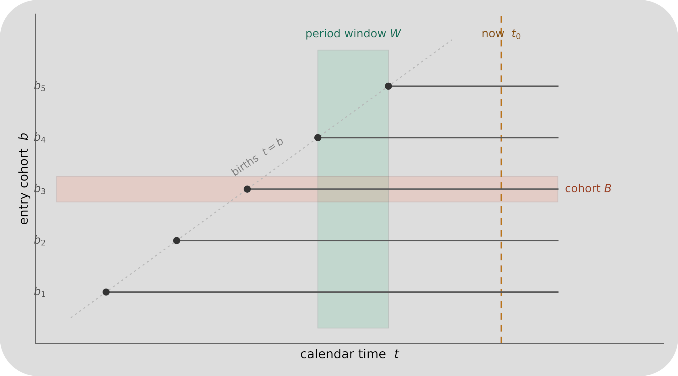
Figure 1. The Lexis domain. Each cohort occupies a horizontal ray beginning on the birth diagonal. A period report is the vertical strip $W$; a cohort report is the horizontal strip $B$; an operational report is the zero-width line at $t_0$.

This is the Lexis diagram, introduced by Wilhelm Lexis in 1875 for exactly this problem in demography: reconciling counts of births, deaths, and populations measured by period against the same counts measured by cohort. The apparatus is 150 years old and has been rigorous for most of them. Business reporting has reinvented the confusion without importing the resolution.

2.1 Two quantity types#

On $L$ we define two distinct kinds of measurement, and the distinction is essential to the discussion:

Stocks. For a cohort set $B$, an instant $t$, and a state $s$:

$$ n(B, t, s) \;=\; \#\{\, i : b_i \in B,\ \sigma_i(t) = s \,\}. $$

A stock is a count of occupancy at an instant. It is defined pointwise in $t$.

Flows. For a cohort set $B$, a time window $W \subseteq \mathbb{R}$, and an ordered state pair $(s, s')$:

$$ f(B, W, s \to s') \;=\; \#\{\, i : b_i \in B,\ \exists\, \tau \in W \text{ with } \sigma_i(\tau^-) = s,\ \sigma_i(\tau) = s' \,\}. $$

A flow is a count of transitions over an interval. It requires $W$ to have positive measure.

Observation 1 (no rates on a snapshot). A flow is undefined on a set of Lebesgue measure zero in the time direction. Any rate, velocity, conversion percentage, or “per period” figure appearing on a report whose time selector is a single instant has been fabricated by the reporting layer — typically by silently substituting a trailing window. This is the most common undetected defect in operational dashboards.

3. The three reports as three cuts#

Every conventional report fixes a region of $L$ and aggregates one quantity type over it. The three families are exactly the three ways to degenerate the two-parameter selection.

Family	Region in $L$	Quantity	Selector
Period / time-domain	vertical strip $\{(b,t) : t \in W\}$	flow	window $W$, all cohorts
Cohort	horizontal strip $\{(b,t) : b \in B\}$	flow or stock	cohort $B$, all time
Operational	vertical line $\{(b,t) : t = t_0\}$	stock only	instant $t_0$

The period report marginalizes over the cohort axis: it counts every transition that happened in $W$, regardless of when the entity entered. The cohort report marginalizes over the time axis: it follows a fixed set of entities forward indefinitely. The operational report marginalizes over both the cohort axis and all history: it reports where everything stands right now and nothing about how it got there.

The three are not competing methodologies. They are projections, and the information each discards is exactly the information the others retain. A period report cannot answer a yield question because it has integrated out the origin. A cohort report cannot answer “how did the business do last quarter” because it has integrated out the period. An operational report can answer neither, and is nonetheless indispensable — it is the fuel gauge.

4. The stability trichotomy#

The three families have different behaviour under re-query, and that behaviour is a complete diagnostic. Let $\rho(\theta)$ denote the value returned by a report when executed at observation time $\theta$, holding the report definition fixed.

Period. For a closed window $W$ with $\theta > \sup W$:

$$ \frac{\partial \rho}{\partial \theta} = 0. $$

The value is constant. Ask again next month, get the same number.

Cohort. For a fixed cohort $B$ and a monotone outcome (e.g. “has converted by $\theta$”):

$$ \frac{\partial \rho}{\partial \theta} \geq 0, \qquad \rho(\theta) \nearrow \rho_\infty \leq |B|. $$

The value is non-decreasing and converges. Ask again next month, get a larger number, converging to a limit.

Operational. $\rho(\theta) = n(\mathcal{E}, \theta, \cdot)$, which is a direct function of $\theta$ with no stability property whatsoever. Ask again during the same meeting, get a different number.

Proposition 1 (report identification). The sign and persistence of $\partial \rho / \partial \theta$ under repeated execution identifies which family a report belongs to, independent of its title, its author’s intent, or its placement on a dashboard.

This is a practical test and it costs nothing: run the report, wait, run it again. It is worth doing because report families are mislabelled constantly, and the mislabelling is invisible until someone divides two numbers that came from different cuts.

Corollary 1 (retroactive mutation detector). If a report is period-family by construction, its window is closed, and yet $\partial \rho / \partial > \theta \neq 0$, then records within $W$ are being mutated after the fact. Common causes: backdated CreatedDate, merge operations that re-parent history, stage fields overwritten without transition logging, and territory reassignment applied retroactively. The magnitude of the drift bounds the volume of retroactive edits.

Corollary 1 converts an annoyance into an instrument. A period report that will not sit still is not a reporting bug; it is evidence about the write path.

5. Yield is a pullback, and it usually does not exist#

The yield question — “how many $Y$ did we get from $X$?” — presupposes a map.

Let $O$ be the set of opportunities and $\Lambda$ the set of leads. Attribution is a partial function

$$ A : O \rightharpoonup \Lambda, $$

assigning to each opportunity the lead it originated from, undefined where no origin is recorded. The yield of a lead set $\Lambda_0 \subseteq \Lambda$ is the cardinality of the preimage:

$$ Y(\Lambda_0) = \left| A^{-1}(\Lambda_0) \right|. $$

Three regimes occur in practice:

$A$ is well-defined and injective on its domain. Yield is unambiguous. Rare, and essentially confined to single-touch, single-product motions.
$A$ is many-to-many (an opportunity sourced by several leads; a lead spawning several opportunities). Then $A$ is not a function and $Y$ requires a choice of allocation rule — first touch, last touch, linear, time-decay, position-based. The number is a property of the rule, not of the business. Reports that do not state the rule are not comparable to each other.
$A$ is largely undefined. The preimage is dominated by the unattributed mass and $Y$ is a lower bound of unknown tightness.

Now the central result. Define transit time $\Delta_i = \tau_i - b_i$, the interval between an entity’s entry and the transition of interest.

Proposition 2 (validity of the naive yield ratio). Let $\Lambda_W$ be the leads created in window $W$ and $O_W$ the opportunities created in $W$. Then
$$ > \frac{|O_W|}{|\Lambda_W|} = \frac{|A^{-1}(\Lambda_W)|}{|\Lambda_W|} > $$
for all $W$ if and only if $\Delta_i = 0$ almost surely.

Sketch. The left side counts opportunities in the vertical strip $t \in W$ regardless of $b$; the right side counts opportunities whose lead has $b \in W$. These agree for every $W$ exactly when no trajectory crosses a window boundary between entry and transition, i.e. when transit time vanishes. $\square$

So the naive ratio is correct precisely in the case where nothing takes any time. Every real pipeline violates the hypothesis, and the error is governed by the dispersion of $\Delta$ relative to the window width: when $\mathrm{sd}(\Delta)$ is small against $|W|$ the ratio is nearly right; when $\Delta$ is comparable to or longer than the window, the ratio is measuring the overlap of two unrelated populations.

This is the formal content of “the 200 are not from the 4,000.” It is not a caution. It is a theorem with a checkable hypothesis, and the hypothesis is false in every enterprise sales motion ever measured.

THE FERRYMAN // Ο πορθμέας
I want to record why this section exists, because it did not come out of a book.
I spent a day with a woman who ran demand generation for a company I was helping. Very good at her work. Quick — quicker than me on her own numbers. And somewhere in the afternoon she got there before I had finished the sentence: that the campaign attribution she reported to her board and the lead sources in the system were never going to agree. Not badly implemented. Never. Not for her, not for anyone, not with more budget or a better tool.
And she cried.
I have thought about that day for years and I have stopped reading it as distress.
She was not upset that she had been wrong. She had understood, faster than the room, that a number she had built four years of work on did not refer to anything. That is not weakness arriving. That is comprehension arriving at speed, and the body does what it does.
I have watched men take the same news by getting loud. Same recognition, different noise. I would not read much into which.
What I take from it is smaller and more useful: she was the only person in that building who ever actually checked. Everyone else had the same broken number and had simply never looked at it hard enough to be hurt by it.
She has hired me four times since. The ones who can stand to find out are the ones worth crossing for.

6. Censoring: cohort reports are biased, and the bias is computable#

The informal advice attached to cohort reports is wait about two years, after which things stop changing. This is a correct observation about the cohort asymptote of Section 4 and useless as guidance, because nobody waits two years.

Formally: for a cohort $B$ with entry time $b$, observed at $\theta$, each entity contributes an observation right-censored at age $a = \theta - b$. Let $\Delta$ be the conversion time, with

$$ P(\Delta < \infty) = p_\infty < 1, $$

since a fraction of any cohort never converts. The distribution of $\Delta$ is therefore defective — its survival function does not decay to zero. This is the standard setting for a mixture cure model:

$$ S(t) \;=\; (1 - p_\infty) \;+\; p_\infty\, S_0(t), $$

where $p_\infty$ is the susceptible (ever-converting) fraction and $S_0$ is a proper survival function for the susceptibles. The observed asymptote is $1 - S(\infty) = p_\infty$: the plateau is the quantity of interest.

The naive cohort estimator at age $a$,

$$ \hat{p}_{\mathrm{naive}}(a) = \frac{\#\{\text{converted by age } a\}}{|B|}, $$

has expectation $p_\infty F_0(a)$, giving relative bias

$$ \frac{\hat{p}_{\mathrm{naive}}(a) - p_\infty}{p_\infty} \;=\; -\,S_0(a). $$

The bias is downward, and it is exactly the susceptible survival function at the observation age — which is estimable from the same data. Fit $S_0$ by Kaplan–Meier on the observed transitions, estimate the plateau, and report

$$ \hat{p}_\infty = \frac{\hat{p}_{\mathrm{naive}}(a)}{\hat{F}_0(a)} $$

with a confidence interval, at 90 days, instead of waiting eight quarters for the number to stop moving.

Two practical cautions. First, identifiability of the cure fraction is weak when follow-up is short relative to the bulk of $F_0$ — the estimate exists but the interval is wide, and reporting the interval is the whole point. Second, if cohorts differ systematically in composition, $S_0$ is not shared across them and must be stratified.

7. The reconciliation identity and the residual as a defect metric#

Stocks and flows are linked by an accounting identity. For a state $s$ and a window $W = (t_0, t_1]$:

$$ n(s, t_1) \;=\; n(s, t_0) \;+\; \beta(s, W) \;+\!\! \sum_{s' \neq s} \!f(s' \to s, W) \;-\!\! \sum_{s' \neq s}\! f(s \to s', W) \;-\; \delta(s, W), $$

where $\beta$ counts entries directly into $s$ and $\delta$ counts departures from the universe entirely — hard deletes, merges, purges, records moved out of scope.

In a system with complete transition logging and no destructive edits, the identity holds exactly. Define the reconciliation residual

$$ \varepsilon(s, W) \;=\; n(s,t_1) - \Big[\, n(s,t_0) + \beta + \textstyle\sum f_{\mathrm{in}} - \sum f_{\mathrm{out}} \,\Big], $$

computed without the $\delta$ term, since $\delta$ is precisely what most CRMs fail to record.

Proposition 3. Under complete transition logging, $\varepsilon = -\delta$. Hence $|\varepsilon|$ is a lower bound on unlogged destructive mutation, and $|\varepsilon| / n(s, t_0)$ is a dimensionless data-quality index for state $s$ over $W$.†

This is the operationally valuable result in the note. “The reports don’t tie out” is normally where the conversation stops. Proposition 3 says the size of the disagreement is itself a measurement — of hard deletes, of merge activity, of stage transitions written directly to the field without a history row, of ownership churn that orphaned its audit trail. Tracking $\varepsilon$ per state per quarter yields a defect surface that localizes which part of the object model is leaking.

8. Non-collapsibility: why segment rates do not average#

Compensation and MBO reports — the wildcard category — combine cuts and segments, and inherit an additional hazard.

Let the population partition into segments $g$ with weights $w_g$ and segment-level conversion rates $c_g$. The aggregate rate is $\sum_g w_g c_g$, which moves when the $w_g$ move even if every $c_g$ is constant. A ratio measure that is not a simple average — an odds ratio, a weighted attainment index, an accelerator multiplier — is non-collapsible: the aggregate is not a weighted mean of the strata at all, and can lie outside their range.

The consequence for compensation design is direct: a plan that pays on an aggregate ratio pays on the segment mix as much as on performance. When the mix shifts for reasons unrelated to the individual — a territory change, a product launch, a pricing change — the plan transfers money for no work. This is Simpson’s paradox in its arithmetic rather than its paradoxical dress, and it is why commission disputes are hard to adjudicate after the fact.

9. Tempo: why period conversion falls when nothing has changed#

The result this note exists to import.

Demography’s sharpest finding on the period/cohort split is the tempo effect. Bongaarts and Feeney (1998) observed that period fertility measures decline when the mean age at childbearing rises, even when completed cohort fertility is unchanged. The period measure confuses a shift in the timing of events (tempo) with a change in their quantity. Their correction, for a period index $Q$ and a rate of change $r$ in the mean timing of the schedule, is

$$ Q_{\mathrm{adj}} \;=\; \frac{Q_{\mathrm{obs}}}{1 - r}, \qquad r = \frac{d\,\bar{\Delta}}{dt}. $$

The business analogue is exact. Let $\bar{\Delta}(t)$ be the mean sales cycle length and $r(t) = d\bar{\Delta}/dt$ its rate of change in dimensionless units (years of cycle length per year of calendar time). Then a period conversion rate observes

$$ c_{\mathrm{obs}}(t) \;\approx\; c_{\mathrm{true}}(t)\,\bigl(1 - r(t)\bigr). $$

If the mean cycle lengthens by 0.2 years per year — a modest deterioration, routinely produced by a move upmarket, an added procurement step, or a new security review — the period conversion rate reads at 80% of true quantum. A 20% apparent collapse in conversion, with no change whatever in the underlying propensity to buy.

The organizational consequence is predictable and expensive: the period number is presented, demand is assumed to have collapsed, and remediation is aimed at the top of the funnel, which is not where anything happened. The cohort measure over the same interval would have been flat.

Two caveats, stated because the correction is easy to over-apply. Bongaarts–Feeney assumes the timing schedule shifts proportionally — the whole distribution slides without changing shape. Compositional change violates this, and the adjusted figure is then not interpretable. And $r$ must be estimated from cohort data; estimating it from period data reintroduces the distortion being corrected.

10. Protocol#

The formal results reduce to six operational rules.

Label every report with its cut. State the cohort selector, the time window, and the quantity type (stock or flow) in the report header. Three fields. A report that cannot be labelled is not a report.
Apply the re-query test to anything whose family is unclear (Proposition 1), and treat drift in a closed-window period report as a finding, not a nuisance (Corollary 1).
Never divide across cuts. A numerator from a period report over a denominator from another period report is a yield claim, and Proposition 2 says it is false unless transit time is zero. Corollary for meetings: present period and operational reports to mixed management audiences and reserve cohort reports for the people doing yield work. This is not condescension — a cohort figure that moves between two meetings will be read as an error by anyone not expecting it to move, and the credibility lost is not recoverable in the same session.
Report cohort yields as cure-model estimates with intervals, not as raw converted-over-total at whatever age the cohort happens to be.
Compute $\varepsilon$ quarterly per state and treat it as a data-quality index (Proposition 3), not as a reconciliation chore.
Estimate $r$ before believing any period-rate decline. If cycle length is moving, the period rate is measuring tempo, not quantum.

Rules 1–3 are free. Rules 4–6 require instrumentation of transition history, which most CRM deployments nominally have and few actually populate. The gap between the nominal and the actual is what $\varepsilon$ measures, which is why rule 5 is the one to implement first: it tells you whether rules 4 and 6 are even computable on your data.

11. Closing#

The informal version of this note has been circulated to clients for years and its practical advice is unchanged: use period reports for results, operational reports for management, cohort reports for yield, and never mix them in one meeting. What the formal treatment adds is that each of those instructions is a consequence rather than a convention, that two of the classic failure modes (naive yield, cohort impatience) have exact corrections, and that the residual everyone treats as noise is a measurement of the system that produced it.

Counting is hard because the object being counted is two-dimensional and every report is a shadow of it. The shadows disagree. That is not a defect in the reports; it is a property of projection. The defect is believing there is a single number.

THE FERRYMAN // Ο πορθμέας
Shadows on a wall, and everyone in the room arguing about which shadow is the horse.
That is not my line, and the man it belongs to has been dead a long time, and he was making a much larger point than I am. I am only saying that a report is a projection, and that a projection throws away a dimension on purpose, and that the thing you cannot see from where you are standing is not gone.
You do not fix a shadow by staring harder at it. You walk round the object.
There is more of this object than I have shown you here. I can feel the edges of it and I do not yet have the words. Something about what is actually being counted, and whether the things in the system are the things in the world at all.
That is a different crossing. Another day.

† The bound is one-sided only in the absence of cancellation. If in-flows and out-flows are both under-logged, their contributions to $\varepsilon$ carry opposite signs and can offset, so a small $|\varepsilon|$ is evidence of clean books only when transition logging is independently known to be complete. In practice the residual should be computed per state rather than in aggregate, since cancellation across states is common and cancellation within a single state’s flow pair is rare.

References#

Bongaarts, J. and Feeney, G. (1998). On the quantum and tempo of fertility. Population and Development Review 24(2), 271–291.

Kalbfleisch, J. D. and Prentice, R. L. (2002). The Statistical Analysis of Failure Time Data, 2nd ed. Wiley.

Kaplan, E. L. and Meier, P. (1958). Nonparametric estimation from incomplete observations. Journal of the American Statistical Association 53(282), 457–481.

Lexis, W. (1875). Einleitung in die Theorie der Bevölkerungsstatistik. Trübner, Strassburg.

Maller, R. A. and Zhou, X. (1996). Survival Analysis with Long-Term Survivors. Wiley.

Vaupel, J. W. (1979). The Lexis diagram: a useful tool. Reprinted discussion in Keiding, N. (1990), Statistical inference in the Lexis diagram, Philosophical Transactions of the Royal Society A 332, 487–509.