Abstract. Customer relationship platforms are commonly described as fracturing their subject matter into silos. We show the fracture is not a schema defect but the composition of two distinct errors: the conflation of a referential layer with an evidential one, and a lossy projection applied to the second. The Lead/Contact division reduces to the definedness of a single partial function and carries no further information. Group interaction, by contrast, is genuinely destroyed: the stored activity set is not a faithful image of the incidence structure that produced it, and no query recovers what the projection discarded. We decompose the observable fraction of an account’s interaction history into three independent factors, give an identifiability condition under which one of them is recoverable by clustering, and bound account coverage from above by capture–recapture. Field correctness is out of scope and treated in the successor note.
Keywords: incidence structures, record linkage, capture–recapture. MSC 05C65, 62D05. JEL C81, M31.
Structure before decay: identity, incidence, and coverage in customer relationship data#
1. Introduction and motivation#
The practitioner complaint about customer relationship platforms is stable across two decades and every vendor: the system sees the world in silos. Leads sit apart from Contacts for no reason a salesperson can articulate. A tradeshow at which nine people from four companies were met resolves into nine unrelated rows. The question how much of this company do we actually know has no answer, and the reporting layer returns silence rather than an error. The genesis of this note is an essay that collects these observations and names the underlying condition entropy.1
The diagnosis is right and the label is premature. Entropy is a statement about a quantity changing over time, and none of the complaints above involve time. They are all present at the instant the data is written. A tradeshow logged this morning has already lost its group structure by lunchtime, not through decay but through the shape of the write. Before one can model how the store degrades, one has to say precisely what the store is a representation of, and where that representation is already lossy on arrival.
That is this note’s scope. It is static throughout. No quantity here has a rate, a half-life, or an equilibrium. We define the entities, the incidence structure over them, the projection that the platform applies when it stores that structure, and the three measurable quantities that bound how much of an account’s history is visible at all. The result is an object with a well-defined notion of completeness. The successor note takes that object and asks what happens to its correctness as the world moves.2
Two claims are worth stating in advance because they cut in opposite directions. The Lead/Contact separation, which generates the loudest complaints, is mathematically trivial — it is the domain and complement of a partial function, and unifying the two loses nothing. The loss of group structure, which generates almost no complaints, is not recoverable in principle from the stored record set. The profession has been irritated by the harmless thing and untroubled by the damaging one.
2. Problem formulation#
2.1 Two layers#
The conventional entity diagram draws Leads, Contacts, Accounts, Opportunities, Events and Campaigns as nodes of a single graph and connects them with a single kind of edge. This is a category error, and it is the source of the tangle. Two distinct kinds of relation are being drawn with one pen.
A schema edge is referential, cardinality-constrained, and timeless. That a Contact belongs to an Account is a fact about the current state of the store, enforced by integrity constraints, with no timestamp and no multiplicity. An evidence edge is an event: it has a time, a channel, a set of participants, and it is never revised, only accumulated. That eleven people sat in a room on 14 March is not a constraint on anything; it is a datum.
We therefore work with two layers over a common vertex set. The schema layer $\mathsf{S}$ carries the referential structure. The evidence layer $\mathsf{E}$ carries incidence. The complaint that the platform cannot show a single stream is, in these terms, the observation that reporting tools query $\mathsf{S}$ and the stream lives in $\mathsf{E}$.
2.2 Identity and the attachment map#
Let $\Pi$ denote the set of persons in the world and $\mathcal{R}$ the set of person-records held in the platform. These are different sets and the platform holds only the second.
Definition 2.1 (Resolution). The resolution map is a function $\theta:\mathcal{R}\to\Pi\cup\{\bot\}$ assigning to each record the person it denotes, or $\bot$ where it denotes no one. The resolved population is $P=\theta(\mathcal{R})\cap\Pi$. Records $r,r'$ are duplicates when $\theta(r)=\theta(r')\in\Pi$.
$\theta$ is not observed. It is the object that record linkage estimates, and every quantity in this note that counts persons rather than rows depends on an estimate of it.3 The duplication factor $d=|\{r:\theta(r)\in\Pi\}|/|P|$ is the correction between row counts and person counts, and it is greater than one in every production system the author has examined.
Definition 2.2 (Attachment). The attachment map is a partial function $\alpha:\mathcal{R}\rightharpoonup\mathcal{A}$ from person-records to accounts. Write $C=\mathrm{dom}\,\alpha$ and $L=\mathcal{R}\setminus\mathrm{dom}\,\alpha$.
The two storage classes the platform exposes are exactly $C$ and $L$. A Contact is a person-record for which $\alpha$ is defined; a Lead is one for which it is not. Qualification — the conversion of a Lead to a Contact — is the extension of $\alpha$ to a record where it was previously undefined.
Proposition 2.3. Let $\upsilon$ be the qualification map, acting on $r\in L$ by defining $\alpha(r)=a$ for some $a\in\mathcal{A}$ and leaving $\theta$ unchanged. Then $\theta$, $P$, and the duplication factor $d$ are invariant under $\upsilon$; and $\alpha\circ\upsilon$ agrees with $\alpha$ wherever the latter is defined.
Proof. Immediate from the definitions: $\upsilon$ modifies only the graph of $\alpha$, adding a pair whose first coordinate lay outside $\mathrm{dom}\,\alpha$. It does not act on $\mathcal{R}$, on $\theta$, or on any existing pair of $\alpha$. $\square$
The content of Proposition 2.3 is negative and that is the point. Qualification changes the definedness of $\alpha$ and nothing else. It follows that the person-level analysis of a book of business should be conducted on $\mathcal{R}$ quotiented by $\theta$, with attachment treated as an attribute that is present or absent, rather than on $L$ and $C$ as separate populations. Any statistic computed on Contacts alone is a statistic conditioned on $\alpha$ being defined — a conditioning that is rarely intended and never declared.
The practical asymmetry that motivates the split is real but lives elsewhere: records in $C$ have generally been through a human check, and records in $L$ have generally not. That is a statement about capture discipline, and capture discipline is a determinant of correctness rather than of structure. It belongs to the successor note.
Figure 1(a) shows the schema layer with the attachment map and its complement made explicit.
2.3 Incidence#
The evidence layer is a hypergraph. An interaction involves a set of people, not a pair.
Definition 2.4 (Incidence). An incidence is a tuple $h=(S_h,\,a_h,\,t_h,\,c_h)$ with participant set $\emptyset\neq S_h\subseteq\mathcal{R}$, account $a_h\in\mathcal{A}\cup\{\bot\}$, time $t_h$, and channel $c_h$. The evidence layer is the multiset $\mathcal{H}$ of incidences. Write $s(h)=|S_h|$ for participant count and $\omega(h)=|\alpha(S_h)|$ for the number of distinct accounts represented among participants for which $\alpha$ is defined.
The interaction taxonomy of the genesis essay is recovered as a classification of $\mathcal{H}$ by the pair $(s,\omega)$, given in Table 1. One category in that essay does not survive the formalisation, and its failure to survive is informative. Additive interaction is not a kind of incidence at all: it is a multiset of pairwise participant-disjoint individual incidences, that is, a property of a collection rather than of a member. Treating it as a fourth type alongside the others is what makes the taxonomy feel unstable. Once it is demoted to an aggregation operator, three genuine classes remain and they are separated cleanly by two binary predicates, $s>1$ and $\omega>1$.
| Class | Participants | Accounts | Instance |
|---|---|---|---|
| Individual | $s=1$ | $\omega\leq 1$ | A call, a one-to-one meeting |
| Group | $s>1$ | $\omega=1$ | A multi-stakeholder meeting at one account |
| Collective | $s>1$ | $\omega>1$ | A tradeshow, a roundtable, a webinar |
Table 1. Classification of incidences by participant count and account multiplicity. Additive interaction is absent by construction: it denotes a multiset of participant-disjoint individual incidences and is a property of a collection, not a class of incidence.
2.4 The storage projection#
Platforms do not store $\mathcal{H}$. They store a set of activity rows, and the shape of that row is decisive.
Definition 2.5 (Storage projection). The storage projection is the map
$$\sigma(h)\;=\;\bigl\{\,(r,\;a_h,\;t_h,\;c_h)\;:\;r\in S_h\,\bigr\},$$extended to collections by $\sigma(\mathcal{H})=\biguplus_{h\in\mathcal{H}}\sigma(h)$.
Each incidence becomes $s(h)$ separate rows, one per participant, each carrying a single participant reference. This is the literal shape of the Salesforce Task and Event objects, whose WhoId field admits one person-record and whose WhatId field admits one related object.4 The co-participation that defined the incidence is not written anywhere.
3. Analysis and method#
3.1 The projection is not injective#
The central structural result is a one-line counterexample, and its triviality should not be mistaken for unimportance. It is the precise form of the claim that no platform can show a single stream.
Proposition 3.1. $\sigma$ is not injective on collections of incidences.
Proof. Fix an account $a$, a time $t$, a channel $c$, and distinct records $r_1,r_2,r_3$. Let $\mathcal{H}_1=\{(\{r_1,r_2,r_3\},a,t,c)\}$, a single incidence with $s=3$. Let $\mathcal{H}_2=\{(\{r_i\},a,t,c)\}_{i=1,2,3}$, three incidences with $s=1$. Then $\sigma(\mathcal{H}_1)=\sigma(\mathcal{H}_2)$, while $\mathcal{H}_1\neq\mathcal{H}_2$. $\square$
Corollary 3.2. Any functional of $\mathcal{H}$ that depends on $s$ is not computable from $\sigma(\mathcal{H})$.
Corollary 3.2 disposes of an entire class of metric. Meeting breadth, multi-threading depth, the number of distinct stakeholders ever in a room together, the ratio of group to individual contact — none of these is a measurement in a platform of this shape. Each is at best an estimate under an assumption that is nowhere stated. This has an uncomfortable consequence for received practice: the belief that multi-threaded opportunities close at higher rates, whatever its merits, is not testable against a store that cannot distinguish a six-person meeting from six calls. The projection does not merely lose the datum. It removes the possibility of checking the doctrine.
Figure 1(b) exhibits the counterexample.
The severity is platform-dependent and honesty requires saying so. Where the activity object admits a set-valued participant association — as engagement-to-contact associations do in some platforms — the hyperedge survives the write and this loss does not arise. Where the participant reference is single-valued, it does. Even under set-valued association the loss reappears through capture discipline, since the participant set is only as complete as the person who attached it; but that is a bounded and improvable loss rather than a structural one.
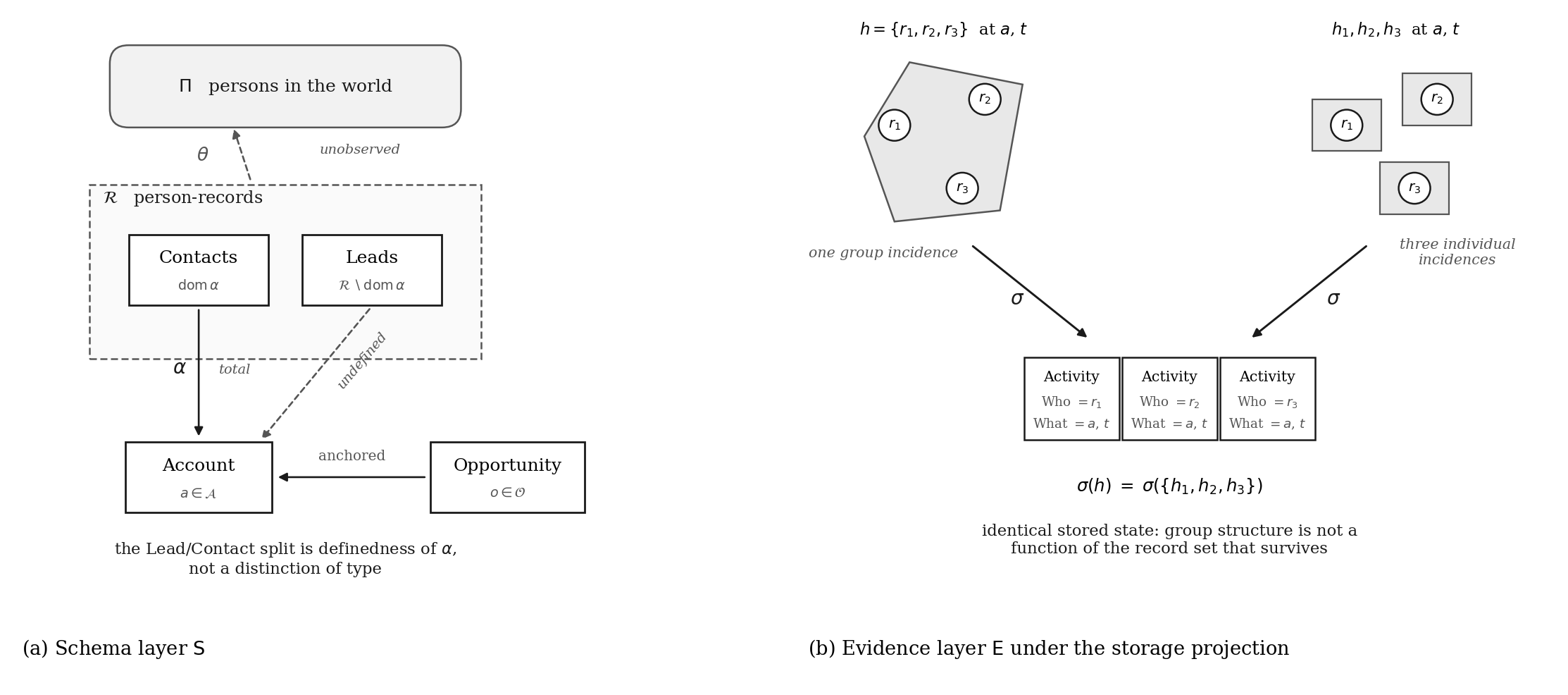
Figure 1. (a) The schema layer, with Leads and Contacts exhibited as the complement and domain of the attachment map $\alpha$; the resolution map $\theta$ to the world is unobserved. (b) Two distinct evidence-layer histories with identical images under the storage projection $\sigma$, establishing Proposition 3.1.
3.2 Recovering incidence by co-occurrence#
The projection is not invertible, but it is invertible under an assumption, and the assumption is testable. Rows sharing an account, a channel, and a sufficiently close timestamp were plausibly one incidence.
Assumption (C). For a given account and channel, at most one incidence occurs within any time bucket of width $\delta$.
Under (C) the fibre of $\sigma$ over the observed rows is a singleton and $\mathcal{H}$ is recovered exactly by grouping. The assumption fails when two genuine incidences collide in a bucket. Model incidences at account $a$ as a Poisson process of rate $\nu_a$, so that the count $N$ in a bucket is Poisson with mean $m=\nu_a\delta$. The probability that a non-empty bucket is ambiguous is
$$\mathbb{A}(\delta)\;=\;\mathbb{P}(N\geq 2\mid N\geq 1)\;=\;1-\frac{m\,e^{-m}}{1-e^{-m}}\;\approx\;\frac{m}{2}\quad(m\ll 1). \tag{1}$$The approximation in (1) is the working form: ambiguity grows linearly in the product of account activity and bucket width, so a bucket may be widened freely at a quiet account and must be kept narrow at a busy one. Figure 3 plots the exact expression.
Widening $\delta$ is not free in the other direction either. Logged timestamps differ from event times by a jitter $J$ — the interval between a meeting and the moment someone wrote it down — and a bucket narrower than the jitter spread splits one incidence into several. The two errors bound $\delta$ from opposite sides.
Proposition 3.3 (Identifiability window). Let $J$ bound the jitter spread and let $\varepsilon$ be a target ambiguity rate. A bucket width satisfying both constraints exists only if $\nu_a J\lesssim 2\varepsilon$.
Proof. Avoiding splitting requires $\delta\geq J$. Bounding ambiguity by $\varepsilon$ requires, via the small-$m$ form of (1), $\nu_a\delta\leq 2\varepsilon$. The interval $[J,\,2\varepsilon/\nu_a]$ is non-empty only under the stated inequality. $\square$
Proposition 3.3 converts a modelling choice into a pre-flight check. Both $\nu_a$ and $J$ are directly measurable from an export — $\nu_a$ from activity timestamps, $J$ from the distribution of the interval between record creation and recorded activity date — so one knows before writing any clustering code whether the accounts of interest admit reconstruction at the desired fidelity. Where they do not, the correct response is to say the metric is unavailable, not to compute it anyway.
Define the structural fidelity $\chi=1-\mathbb{A}(\delta)$ as the fraction of incidences correctly reconstructed at the chosen bucket width.
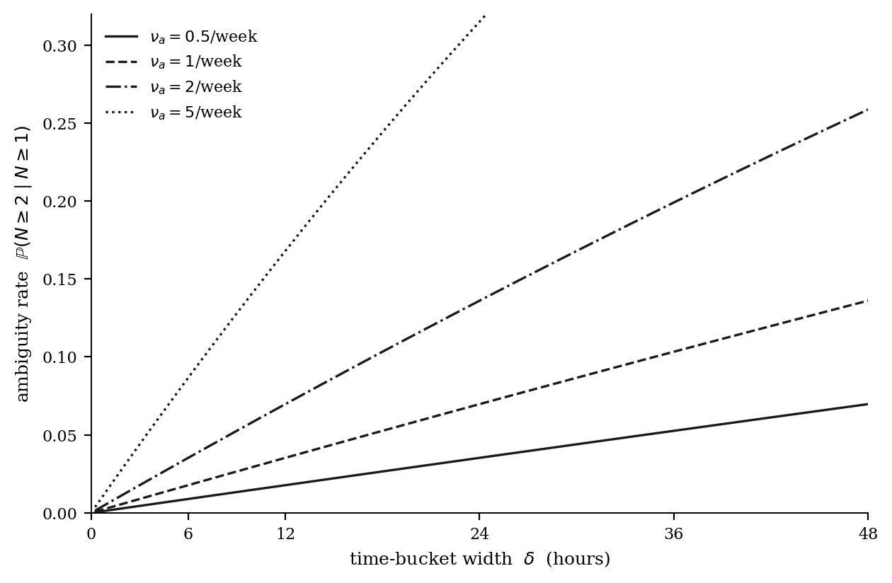
Figure 3. Ambiguity rate from (1) against time-bucket width, for four account activity rates. At two incidences per week a daily bucket leaves roughly fourteen percent of non-empty buckets ambiguous; at five per week the same bucket is unusable.
3.3 The stream and its completeness#
The single stream that the genesis essay asks for is now definable.
Definition 3.4 (Account stream). The stream of account $a$ is the time-ordered restriction of the evidence layer to incidences touching the account, $\Sigma_a=\{h\in\mathcal{H}:S_h\cap\alpha^{-1}(a)\neq\emptyset \text{ or } a_h=a\}$, ordered by $t_h$.
$\Sigma_a$ is a well-defined object over $\mathsf{E}$. What the platform holds is an estimate $\hat\Sigma_a$ obtained from stored rows, and the gap between them decomposes into three independent mechanisms.
The first is capture: an incidence that no one logged is absent regardless of everything else. Write $\beta$ for the fraction of true incidences that reach the store at all. The second is attribution: a logged incidence whose participants all have $\alpha$ undefined cannot be placed against any account, and falls out of every account stream. Write $\eta$ for the fraction of logged incidences attributable to an account. The third is structure, the fidelity $\chi$ of Section 3.2.
Proposition 3.5 (Loss decomposition). If the three mechanisms act independently, the expected observed fraction of the true stream is $F=\beta\eta\chi$. In general $F$ obeys the Fréchet bounds
$$\max\bigl(0,\;\beta+\eta+\chi-2\bigr)\;\leq\;F\;\leq\;\min(\beta,\eta,\chi). \tag{2}$$
Proof. The product form is the independence case. The bounds in (2) are the Fréchet–Hoeffding bounds applied to the joint occurrence of the three retention events.5 $\square$
The dependence is not neutral in practice and its direction is favourable. Interactions with unattached leads are also disproportionately the interactions nobody logs, so the retention events are positively associated and the true $F$ generally exceeds the product. The product is therefore a conservative estimate, which is the correct posture for a diagnostic that will be shown to a prospect.
Figure 2 renders the cascade with illustrative factors. The arithmetic is unremarkable and the conclusion is not: three individually tolerable retention rates compose to a stream that is roughly a third of the truth.
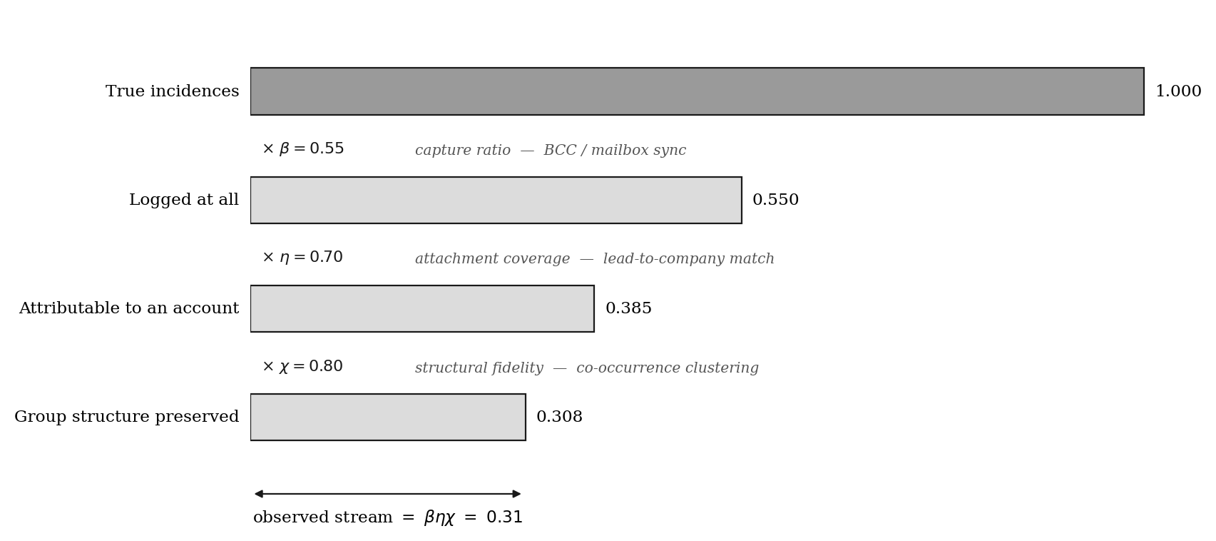
Figure 2. Multiplicative decomposition of stream completeness with illustrative factors. Each factor has a distinct remedy and the remedies are orthogonal; no one of them addresses more than its own term.
3.4 Coverage of an account#
The question how much of this company do we know asks for the ratio of persons held to persons who matter. Let $B_a$ denote the size of the buying group at account $a$ and let $n_a=|\theta(\alpha^{-1}(a))|$ be the number of distinct persons held against it after deduplication. Coverage is
$$\kappa_a=\frac{n_a}{B_a}. \tag{3}$$The numerator of (3) is computable and the denominator is not observed, which is why the platform returns silence. But $B_a$ is estimable, and the estimator is standard in a literature the profession has not consulted: capture–recapture. It requires two partially independent enumerations of the same population, and the two-layer model supplies exactly that. The first source is the schema layer — person-records attached to $a$, count $n_1$. The second is the evidence layer — distinct human counterparties appearing in incidences at $a$, count $n_2$ — which sees people who correspond with the firm without ever having been entered as records. Let $m$ be the overlap. The Chapman estimator and its variance are
$$\hat B_a=\frac{(n_1+1)(n_2+1)}{m+1}-1,\qquad \hat V=\frac{(n_1+1)(n_2+1)(n_1-m)(n_2-m)}{(m+1)^2(m+2)}. \tag{4}$$Chapman’s form in (4) is preferred to the ratio estimator because it is nearly unbiased at the small overlaps typical of a single account.6 Its assumptions are closure of the population over the observation window, independence of the two captures, and homogeneous capture probability. All three are violated to some degree, and the direction of the resulting bias matters more than its size.
Capture dependence is positive: a person entered as a record is more likely, not less, to appear in logged correspondence. Positive dependence inflates the overlap $m$, which deflates $\hat B_a$, which inflates $\hat\kappa_a$. Heterogeneity of capture acts the same way.
Proposition 3.6. Under positive capture dependence or heterogeneous capture probability, $\hat\kappa_a$ computed from (3) and (4) is biased upward. It is therefore reportable as an upper bound on coverage, not as a point estimate.
Proof. Both conditions raise $\mathbb{E}[m]$ relative to the independent-homogeneous case; $\hat B_a$ is decreasing in $m$ and $\hat\kappa_a=n_a/\hat B_a$ is decreasing in $\hat B_a$. $\square$
This is the strongest honest claim available and it is strong enough. One cannot tell a prospect what fraction of the buying group they know. One can tell them it is at most some number, with a stated interval, and that bound is derived rather than asserted. Where several observation windows are available, Chao’s lower bound on population size under unequal catchability provides the heterogeneity-robust alternative and preserves the direction of the inequality.7
3.5 Outcome attachment#
Opportunities anchor to accounts, and the question of which interactions produced them is an attribution problem defined on the stream: for opportunity $o$ at account $a$ created at $t_o$, the antecedent set is $\Sigma_a\cap\{h:t_h The genesis essay lists three remedies — mailbox capture, automatic lead-to-company matching, and activity clustering — and dismisses them as band-aids over a fundamentally broken system. The decomposition in Proposition 3.5 says otherwise. They are not palliatives applied to a single wound. They are three instruments, each acting on exactly one factor of a product, and together they exhaust the structural loss. Table 2. The three factors of stream completeness, the instrument acting on each, and the data required to measure it. Orthogonality is the useful property. Perfect matching does not recover an unlogged meeting; perfect capture does not attribute a lead to a company; neither reconstructs a hyperedge from single-participant rows. A programme that installs one and expects the stream to improve threefold has misread the arithmetic. What the table does not contain is any instrument acting on whether the fields of a retained record are correct, because no such loss appears in this note. That is the successor’s subject and the boundary is clean. A single CRM export, with mailbox metadata where available, supports the following without access to any system of record beyond the client’s own. $\eta$ is immediate: the fraction of person-records with $\alpha$ defined, corrected for duplication by $\theta$. $\nu_a$ and $J$ follow from activity timestamps and the interval between record creation and recorded activity date; together with a chosen $\delta$ they give $\chi$ through (1), and Proposition 3.3 says whether the chosen $\delta$ is admissible at all. $n_1$, $n_2$ and $m$ per account give $\hat B_a$ and hence the coverage bound through (3) and (4). $\beta$ is different and the difference should be stated rather than finessed. The platform cannot see interactions the platform never received. No statistic computed on stored rows estimates the fraction of interactions absent from those rows; the quantity is unidentifiable without an independent capture source. This is not a limitation of the method but of the data, and it has a direct operational consequence: mailbox capture is not merely the instrument that improves $\beta$, it is the only instrument that makes $\beta$ observable. Until it is in place, stream completeness is reportable only as $F\leq\eta\chi$. Consider one account, with figures chosen to be plausible rather than drawn from a client.8 The schema layer holds $n_1=6$ attached person-records after deduplication. The evidence layer shows $n_2=11$ distinct human counterparties at the account’s domain, of whom $m=4$ correspond to held records. Chapman’s estimator (4) gives $\hat B_a=15.8$ with $\widehat{\mathrm{Var}}=7.84$, so $\mathrm{SE}=2.8$ and a nominal 95 percent interval of $[10.3,\;21.3]$. Coverage follows: $\hat\kappa_a=6/15.8=0.38$, with the interval $[0.28,\,0.58]$ obtained by inverting the endpoints. By Proposition 3.6 the whole interval is an upper bound. The defensible statement to the account owner is that they hold at most somewhere between a quarter and three-fifths of the relevant buying group, and most likely nearer the lower end — from a single account, on their own data, with no vendor enrichment. The interval is wide because one account is a thin sample; aggregating the estimator across accounts of similar size tightens it considerably, at the cost of assuming homogeneity of $B$ within the stratum. Taking $\nu_a=2$ per week and $\delta=24$ hours, (1) gives an ambiguity rate of $0.136$ and hence $\chi=0.86$; with $\eta=0.60$ at this account, the observable stream is bounded by $\eta\chi=0.52$ before any allowance for unlogged interaction. Slightly more than half the account’s history is visible in the best case, and the best case assumes every interaction was logged. The identity map $\theta$ is unobserved and every person-count in this note inherits the error of whatever linkage procedure estimated it. Duplicates inflate $n_1$ and $m$ together, and the net effect on $\hat B_a$ is not signed in general; deduplication must therefore precede capture–recapture rather than follow it, and a sensitivity analysis over plausible linkage thresholds should accompany any coverage figure that leaves the building. Capture–recapture assumes a closed population over the observation window. Buying groups change composition, so the window must be short relative to the timescale on which they turn over. Quantifying that timescale requires a decay model and is deferred. The evidence layer as construed here is channel-specific. Mailbox capture sees email and not telephone calls, corridor conversations, or the parts of a tradeshow that happened away from a scanner. Consequently $\beta$ is properly a vector indexed by channel, and a single scalar reported without naming the channel is a category error of the same kind this note began by identifying. Where a channel is structurally uncapturable, the honest treatment is to exclude it from the denominator and say so. There is a legal bound on the observation window that has no technical counterpart. Retaining counterparty interaction metadata is processing of personal data; in the EU it is generally conducted under the legitimate-interest basis of GDPR Art. 6(1)(f), subject to a balancing test, and is constrained by the storage-limitation principle of Art. 5(1)(e). The practical consequence is that the window over which $\beta$, $\nu_a$ and the capture–recapture sources may be assembled is set by a retention policy rather than by data availability, and a coverage estimate whose window exceeds the client’s own retention schedule is not merely inadmissible but embarrassing.9 Finally, the model takes the account as the correct anchor. Corporate groups with subsidiaries break $\alpha$ into a hierarchy, and coverage computed at the wrong level of that hierarchy is not wrong so much as answering a different question. Where the hierarchy is present in the store, $\kappa$ should be reported at each level it is asked about. The tangle in customer relationship data is two errors compounded, and they are of very different weight. Drawing referential and evidential relations on one diagram makes the schema look incoherent when it is merely being read at the wrong layer; separating the layers dissolves the Lead/Contact problem entirely, since that division is nothing but the definedness of a partial function and unification costs nothing. Storing a hypergraph through a single-participant projection, by contrast, destroys information that no query recovers, and the profession has been remarkably calm about it. What survives the analysis is a definite object. An account’s stream is well defined on the evidence layer, its observable fraction factors into capture, attribution and structural fidelity, and two of those three factors are measurable from an export the client already possesses. Coverage cannot be measured but can be bounded above, by an estimator that has been standard in population ecology for seventy years and requires only the two enumerations the two-layer model already provides. That is a smaller claim than the genesis essay’s, and it has the advantage of being true. None of this has involved time. Every quantity here would take the same value if the world stopped the moment the export was taken. The store is already incomplete on arrival, and the incompleteness is structural, bounded, and instrumentable. What happens next — the movement of the world away from a record that does not move with it — begins where this note ends. Berge, Claude. Hypergraphs: Combinatorics of Finite Sets. Amsterdam: North-Holland, 1989. Chao, Anne. “Estimating the Population Size for Capture-Recapture Data with Unequal Catchability.” Biometrics 43, no. 4 (1987): 783–791. Chapman, Douglas G. “Some Properties of the Hypergeometric Distribution with Applications to Zoological Sample Censuses.” University of California Publications in Statistics 1, no. 7 (1951): 131–160. Fellegi, Ivan P., and Alan B. Sunter. “A Theory for Record Linkage.” Journal of the American Statistical Association 64, no. 328 (1969): 1183–1210. Nelsen, Roger B. An Introduction to Copulas. 2nd ed. New York: Springer, 2006. §2.5. Penrose, Edith. The Theory of the Growth of the Firm. Oxford: Blackwell, 1959. Seber, George A. F. The Estimation of Animal Abundance and Related Parameters. 2nd ed. London: Griffin, 1982. Ch. 3. G. Righter, “The Entropy of Business Data: A Predecessor Story,” ZnuLabs working manuscript, 2026. The historical material in that essay — the postal acts, the publisher list lineage, Siebel’s automation of the pipeline — is not reproduced here and is not required by the argument. Its value is in establishing that the list, not the relationship, is the ancestor of the schema, which explains why the schema anchors on the record rather than on the person. ↩︎ TN-2026-002, “The thermodynamics of business data: decay, injection, and the economics of standing remediation.” Symbols in the present note are chosen to avoid collision with that one wherever a quantity is load-bearing in both: $\theta$ for resolution rather than the remediation rate, $\nu$ for incidence arrival rather than the turnover rate, $s$ and $\omega$ for incidence dimensions rather than the per-field and inflow qualities. Two overlaps remain and are disambiguated by context: $a$ denotes an account here and the anchorable fraction there, and $N$ denotes a bucket count here and the base size there. ↩︎ The estimation of $\theta$ is the record linkage problem in its classical form; the probabilistic framework of Fellegi and Sunter (1969) remains the reference treatment, and the comparison-vector machinery there is what a modern deduplication routine implements under other names. ↩︎ Salesforce, Object Reference for the Salesforce Platform, s.v. “Task” and “Event,” fields The bounds are the standard Fréchet–Hoeffding bounds on a joint distribution given its margins; see Nelsen, An Introduction to Copulas, §2.5. Applied here to three indicator variables they reduce to the elementary Bonferroni inequality, which is how they are used above. ↩︎ The naive Lincoln–Petersen ratio $n_1n_2/m$ has infinite expectation when $m=0$ and substantial small-sample bias for the overlaps typical of a single account. Chapman’s modification is nearly unbiased provided $n_1+n_2\geq B$; see Seber, The Estimation of Animal Abundance, Ch. 3. ↩︎ Chao (1987) gives $\hat B\geq n_{\mathrm{obs}}+f_1^2/(2f_2)$ where $f_1$ and $f_2$ are the numbers of persons observed exactly once and exactly twice across capture occasions. As a lower bound on $B$ it yields an upper bound on $\kappa$, preserving the direction of Proposition 3.6. ↩︎ The figures in Section 4.3 are illustrative and chosen for plausibility. They are not drawn from any client engagement and should not be cited as an empirical result. ↩︎ Regulation (EU) 2016/679, Arts. 5(1)(e) and 6(1)(f). This is a statement of where the constraint sits in the architecture, not legal advice; the balancing test under Art. 6(1)(f) is fact-specific and national supervisory practice varies. ↩︎4. Results and interpretation#
4.1 Three losses, three instruments#
Loss channel Factor Instrument Measurable from Interaction never logged $\beta$ Mailbox and calendar capture Not estimable from the platform alone Participants unattached to any account $\eta$ Lead-to-company matching Directly, from definedness of $\alpha$ Group structure collapsed by the write $\chi$ Co-occurrence clustering at width $\delta$ $\nu_a$ and $J$ from activity timestamps 4.2 What is measurable from an export#
4.3 Worked illustration#
5. Implications and limitations#
6. Conclusion#
References#
WhoId and WhatId. WhoId references a single Lead or Contact. The EventRelation object permits multiple invitees on an Event and is a partial exception, but it is not populated by the majority of logging paths — in particular not by email logging — so the projection of Definition 2.5 describes the dominant case rather than the only one. ↩︎